? Practical skills assessed in a written examination (FREE TO VIEW)

The A Level Biologist - Your Hub February 24, 2020
Planning
Variables
Variables are factors present in an experiment. Often, they are the factors that we are primarily interested in e.g. testing a food variable against an age variable. Due to the nature of experiments taking place in the actual world, many confounding variables can present themselves, more or less clearly, in experiments. Confounding variables are those variables which can overlap so that it cannot be obvious whether a result is due to one variable or another. For example, in looking at people’s diets which contain both fat and sugar, these components are confounding variables of each other in a study that wants to only look at the effect of fat or sugar.
In order to tease away confounding variables from each other, a technique called randomised block design is used to categorise data into groups, and then carry out the experiment independently in each. For example, participants can be split by weight, diet, sex, height, etc. so that any findings can be said to not be due to any of these pre-split factors.
Variables vary by the type of data they can produce. Discrete variables give rise to individual data points that cannot be connected e.g. colours, whole numbers of things, blood groups. Continuous variables give rise to data that is possible on a spectrum of connected values e.g. height, width, solute concentration.
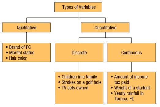
As such, the data derived can be qualitative (green, blood group B), quantitative (1.55 m, 65 nm, 50 nM NaCl) or ranked (low, moderate, high intensity).
Different data can be displayed and analysed in different ways – graphically, statistically, etc. Data can be represented in many ways e.g. bar charts, scatter plots, images, photos, tables. The type of data determines what method can be used to represent and analyse it.
Experimental design
Experimental design covers the equipment and reagents needed and whether these are safe and cost-effective enough to justify their use; what experiments will be carried out, when, in what order, how and how many times; what data will need to be recorded; what biases might arise and how to counteract them e.g. labelling tests using codes rather than content names; how to organise experiments to fit with experimenter’s schedules or equipment booking schedules; how to collect the right amount of data from experiments to be able to use certain statistical tests afterwards i.e. some tests need a minimum of data to apply.
Things to consider during the process of developing an experimental design are the controls, dependent and independent variables. Controls are experiments that establish a baseline or use a default, standard or neutral state to ensure the actual test experiment doe not merely produce background results, or results that are not due to the tested variable.
Dependent variables are the target variables – these are observed against the independent variable to check what is happening. The independent variable is a known variable that can be a constant e.g. time, distance, concentration. The dependent variable is what is tested against it e.g. colour, substrate breakdown, growth.
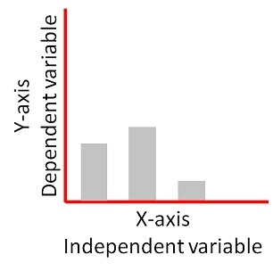
As such, the independent variable is controlled and set up by the experimenter to be able to test and observe the progress of the dependent variable against it.
Simple experiments use one independent variable only. These are often carried out in vitro i.e. in the lab using simple reagents like chemicals or cells. The downside to these relatively easier, more straightforward experiments is that their findings may not be as applicable to a wider real life context as in vivo experiments. These are carried out in living organisms.
Complex experiments, such as those in vivo, present multifactorial experimental designs. They have more confounding variables, including independent variables.
In observational studies, there is no independent variable, as groups already exist in the wild as they are. These studies can reveal correlations between variables, but are less useful for revealing causation.
Controls
Positive and negative controls are used for experiments. Controls ensure that the outcome of the experiment is what it seems to be.
Positive controls give a reference point for what the result would look like if it worked, while negative controls give a reference point for what the result would look like if it didn’t work.
A positive control for PCR might be a PCR reaction identical to the one we are running as an experiment, but instead of the test template DNA we add a different template DNA that we know will definitely work based on previous data. If the experiment fails, but the positive control works, we can be sure that the PCR reaction was correct but there was an issue with the test template DNA.
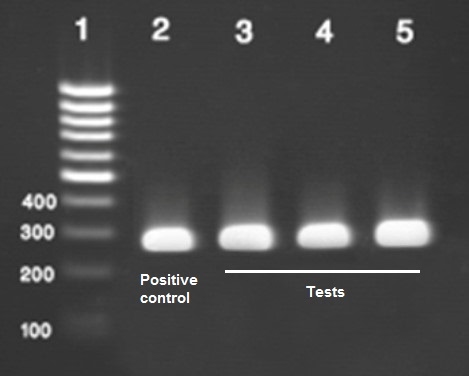
A negative control for PCR requires a little less sophistication, and might involve using the same PCR reaction while omitting any template DNA at all. If we seem to get something that looks like it worked in our experiment using our template DNA, but it looks the same as the negative control, then we can be sure that it actually hasn’t worked, and the result is because of another reason e.g. contamination, background signal, PCR ingredients themselves, etc.
Sampling
When sampling things from the field, it is key to ensure representative sampling. This depends on the variability in the population. The more variable a population, the larger the sample would have to be in order to be representative.
The mean of, and variation around a sample should closely match those of the actual population. It is impractical to aim to collect each member of a population, so sampling is necessary.
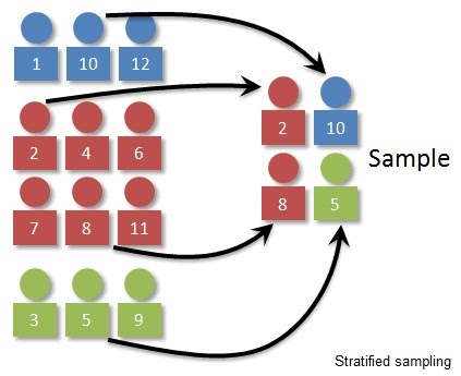
Random sampling involves an equal probability of any member of the population being chosen. Systematic sampling involves sampling that takes place at intervals e.g. using transects. Stratified sampling involves splitting the population into categories and then sampling from the categories. This is useful when these categories already exist, or there is a reason why they might be confounding variables unless split, as seen in randomised block design.
Implementing
Once the experimental design is in place, the implementation involves simply carrying out the steps in the experiment as planned. Many techniques such as microscopy, sampling, enzyme reactions and electrophoresis are covered in their respective topics across the specification.
Obtaining results is the next step. This involves first collecting the data which as previously mentioned, might start right from the experimental design step because sometimes the data might be missed unless specifically waited on to be collected. Sometimes an experimenter might have a split second to collect the data, else the experiment is wasted. This must be planned for in advance. Sometimes equipment collects data automatically in which case one can take a nap.
Either way, once collected, data is kept in a store (whether physical or digital) as raw data. This is then looked at and analysed using various methods such as computing, graph generator software, image processors, etc.
It is crucial to know what units the data needs to be measured in. For example, if we are looking at the rate of reaction of an enzyme-catalysed reaction, we would monitor the amount of substrate used up, or amount of product made, over time. If the reaction is quick, we might need to measure it every 10 seconds and report it in amount per second, for example. It would be totally inappropriate to measure it in amount per millisecond or per hour. This is because the former would be impossible to measure anyway, while the latter would completely miss the reaction taking place (perhaps after an hour it has finished, and we missed the active reaction).
Equally, variables have respective units. Mass is milligrams, while density (= mass / volume) would be milligrams per cm3, or grams per litre. Various variables in different contexts have different units, depending on how much there is, what a tool can measure, how fine the data needs to be for analysis or drawing conclusions, etc. Use common sense.
Analysis
Evaluation of results involves fitting the new data into the existing knowledge. Sometimes this involves discarding what is outlier data, running additional statistical tests to fine tune results, dealing with unexpected results, or outright finding out that the experiment didn’t run as intended.
Examples of analyses run on data include calculating means and standard deviations, running statistical tests to determine whether a difference is statistically significant, adjusting raw data to make it comparable between groups, etc.
Significant figures must be used correctly, too. Significant figures in a number represent the necessary degree of accuracy starting from the first non-zero digit. For example, weight might be accurate enough to 2 or 3 significant figures. For a human, 2 sig. fig. of 60 kg or 73 kg might be sufficient. If weighing potassium chloride for a solution, 3 sig. fig. might be necessary e.g. 6.24 g instead of just 6.2 g.
It would be entirely useless to display people’s height to 1 sig. fig. and obtain heights of 1 metre. Everyone could be 1 metre. Therefore, 2 sig. fig. (1.2 m, 1.6 m, etc.) is better, and 3 sig. fig. is ideal (1.26 m, 1.65 m, etc.).
The processed data is then displayed in tables, graphs, images, etc. Different types of data e.g. qualitative or quantitative are displayed using different methods. For example, microscopy data (qualitative) consists of images. Sometimes these must be edited or data extracted from them e.g. number of cells (quantitative). This must be done carefully to avoid creating image artefacts or manipulating the images beyond what they actually show.
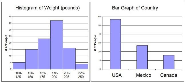
Bar charts are used for discrete data, while histograms are used for continuous data. Presented data can be displayed in any way that is useful.
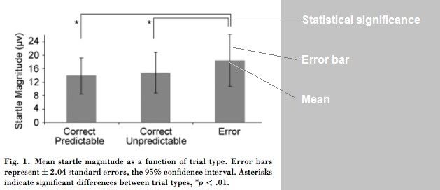
Many data analysis and representation practices exist that have become popular and are used as conventions. For example, statistical significance is represented by an asterisk, while the mean and standard error are represented with a capped line.
As you can see, graphs have certain essential elements e.g. two axes (x axis and y axis), one horizontal and one vertical. These must be labelled with the correct variables and units. In this example the axis labels are “Startle Magnitude” and trial type. Note that trial type isn’t actually labelled on the x axis… It contains the categories “Correct Predictable, Correct Unpredictable and Error”.
The y axis uses micro Volts (μV) as the unit for startle magnitude. The x axis categories do not require units because they are not quantitative.
The graph has a numbered (Fig. 1) and descriptive caption. The range used on the y axis is appropriate (0 – 24 μV) because is covers the data and the standard error. For example, if the axis only went up to 20 μV, it would not include the upper standard error of the last bar.
Finally, the statistical significance relationships between trial types is displayed correctly (if present; not all data include statistical analysis) through the use of connecting lines and asterisks.
Once we have a graph, many useful details can be extracted from it, such as line gradients and intercepts.
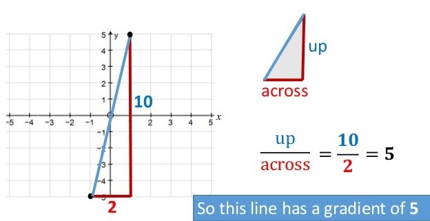
A gradient represents the relative position of a line on the x and y axes, that is how steep the line is. It is calculated by dividing the distance it spans along the y axis by the distance it spans along the x axis. The shape is a triangle and works out the same either direction.
Intercepts are points where a line meets the x axis or the y axis. For example, the line in the gradient example intercepts both axes at 0. This gives that point coordinates of (0, 0).
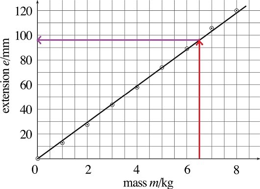
Intercepts are useful at finding information from a linear graph by drawing a line from the point of interest (what’s the extension value for a mass of 6.5 kg?), perpendicularly to the line of best fit (red arrow), and then towards the other axis (purple arrow) to find the target value (96 mm).
Evaluation
The experimental design must be adequate for testing the stated hypothesis and aims. Appropriate controls and treatments, as well as steps to deal with confounding variables must have been taken.
If a sample was taken, the effects of sampling bias and whether it was representative must be considered.
In the results section, the suitability of graphs used must be assessed as well as the use of different statistical tests. A low sample might not have sufficient statistical power to warrant the use of a statistical test. Statistical significance refers to the outcome of a statistical test that indicates the result in question is unlikely to have occurred merely by chance. It is often used as a litmus test for “proving” that something is happening in the data presented.
This is to be considered with caution. Probability is by convention set at 5% (p value = 0.05), meaning that as long as a statistical test outcome gives a probability of the result happening due to chance less than 5%, then the result is considered statistically significant. This leaves a loophole for results not always being what they are supposed to be. Additionally, there are fields or types of data that cannot subscribe reliably to the use of certain statistical tests.
Statistical tests are just mathematical tools that deal with probability, and as such cannot guarantee or create knowledge in their own right.
Means used in graphs in the results section of a paper have confidence intervals or error bars around them, indicating how wide the rest of the data is dispersed around the mean. This shows data variability and is also used to compare sets of data side by side. If their means with error bars overlap, they are similar. Non-overlapping means and error bars, especially with statistical test significance (as previously mentioned) imply a difference between data sets.
As for conclusions, they should refer to the original aim and hypothesis. In assessing the conclusion, the validity (does the data reflect what was intended to be measured?) and reliability (would this data occur again if the experiment were repeated?) of the experimental design must be accounted for.
Ensuring reliability
Reliability refers to the extent to which the same results would be obtained if an experiment were repeated independently. Data collected must be reliable. If variation is found in data, it is critical to know whether this is because of the data itself, or due to the measuring technique, equipment, human handling, etc.
Repeated measurements have two key properties: precision and accuracy. Precision refers to the inherent statistical variability data can be expected to have; while accuracy refers to the closeness of data obtained to the actual “real” value it is supposed to represent.
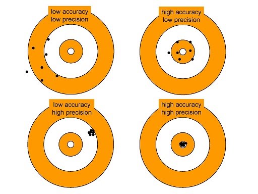
Data can be very precise but off the mark of the actual things that are happening in the experiment. Data can also be accurate in terms of representing what is happening in the experiment, but lack precision.
Very precise but not accurate data reflects a systematic error e.g. broken instrument that no longer measures its variable, but still outputs precise data points referring to a non-existent phenomenon.
Accurate but imprecise data reflect a random error where the data do represent the real phenomenon that is happening, but the measurements have random errors that impact precision.
Means are used to pool these variable data points to obtain a true reflection of the overall measured phenomenon.
Reliability can be checked by repeating whole experiments. Reliable experiments and data should play out the same way as originally, while unreliable data could even be impossible to reproduce. Many technically complex, expensive experiments e.g. Large Hadron Collider experiments are likely to not be reproducible for some time, or by certain people or countries, or ever.
Finally, thought must be given to whether the connections made by the results are correlation or causation. Statistical significance gives confidence to the divergence of sets of data, but cannot provide explanation or what might have created that data. The balance between the data and its analysis, and the wider narrative of the field must be merged artfully to understand reality and contribute to the advancement of new knowledge.
Ok byeeeeee